Difference between revisions of "Automatic DBS lead topology correction"
| (4 intermediate revisions by the same user not shown) | |||
| Line 11: | Line 11: | ||
By wireframe path, I mean a piecewise linear curve in 3D space that represents the centerline path of the DBS lead. Every segment is linear and the wireframe path model is therefore simply defined by a set of ordered points in 3D space. | By wireframe path, I mean a piecewise linear curve in 3D space that represents the centerline path of the DBS lead. Every segment is linear and the wireframe path model is therefore simply defined by a set of ordered points in 3D space. | ||
| − | I refer to this process of enforcing (i) a minimum distance between any two segments of the path and (ii) a maximum curvature at every point of the path as "topology correction". This is because if the two segments are too close to each other (distance constraint violation) or if the path bends too quickly (curvature constraint violation), once the path is thickened to the actual lead diameter this will result in self-intersections of the cable model. This topology correction process is formulated as a constrained optimization problem solved using an active-set approach. The technique is accelerated using a GPU, but even then computation is relatively slow: Count a few | + | I refer to this process of enforcing (i) a minimum distance between any two segments of the path and (ii) a maximum curvature at every point of the path as "topology correction". This is because if the two segments are too close to each other (distance constraint violation) or if the path bends too quickly (curvature constraint violation), once the path is thickened to the actual lead diameter this will result in self-intersections of the cable model. This topology correction process is formulated as a constrained optimization problem solved using an active-set approach. The technique is accelerated using a GPU, but even then computation is relatively slow: Count a few minutes for a lead with ~300 points. |
=== Download files === | === Download files === | ||
| − | The code, examples and additional scripts for creation of DBS leads in HFSS can be downloaded [https://ptx.martinos.org/images/ | + | The code, examples and additional scripts for creation of DBS leads in HFSS can be downloaded [https://ptx.martinos.org/images/0/09/DBS_RemoveLead_Intersections_WEB.zip here]. |
=== Instructions === | === Instructions === | ||
Download the zip file using the link above and unzip it. | Download the zip file using the link above and unzip it. | ||
| − | |||
| − | |||
| − | |||
| − | |||
| − | |||
==== Running an example ==== | ==== Running an example ==== | ||
| − | The subfolder EXAMPLE/ contains an example of how to run the code. The master script is | + | The subfolder EXAMPLE/ contains an example of how to run the code. The master script is RUN_OPT.m. All the options used in this script are commented and should be easy to understand. There are several things to note in this script: |
* Both the left and right DBS leads are loaded in Matlab and are connected in a single wireframe dataset. The topology correction process is run on this "super-lead" in order to remove gamma distance violations not only between the segments of a given lead, but also between segments belonging to different leads. Once the topology correction has been performed, the left and right leads can be separated again. | * Both the left and right DBS leads are loaded in Matlab and are connected in a single wireframe dataset. The topology correction process is run on this "super-lead" in order to remove gamma distance violations not only between the segments of a given lead, but also between segments belonging to different leads. Once the topology correction has been performed, the left and right leads can be separated again. | ||
| − | + | * The topology correction process itself is performed by the Matlab function deform_path_LINEAR.m. | |
| − | * The topology correction process itself is performed by the Matlab function deform_path_LINEAR.m | ||
| − | |||
| − | |||
| − | |||
| − | |||
| − | |||
| − | |||
==== Additional scripts ==== | ==== Additional scripts ==== | ||
Latest revision as of 16:57, 19 March 2018
Citation
Coming up soon.
What this code does
This codes takes as input a wireframe model of a DBS lead and returns in output the wireframe model that is the closest to the initial path (in the L2 sense) but for which:
- The distance between any two segments of the path is greater than Dmin, where Dmin is a distance defined by the user.
- At every point of the path, the curvature is smaller than Kmax, where Kmax is the maximum curvature defined by the user.
By wireframe path, I mean a piecewise linear curve in 3D space that represents the centerline path of the DBS lead. Every segment is linear and the wireframe path model is therefore simply defined by a set of ordered points in 3D space.
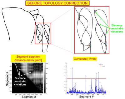
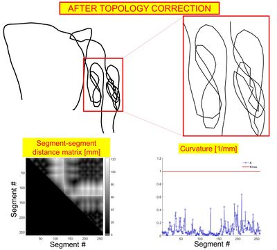
I refer to this process of enforcing (i) a minimum distance between any two segments of the path and (ii) a maximum curvature at every point of the path as "topology correction". This is because if the two segments are too close to each other (distance constraint violation) or if the path bends too quickly (curvature constraint violation), once the path is thickened to the actual lead diameter this will result in self-intersections of the cable model. This topology correction process is formulated as a constrained optimization problem solved using an active-set approach. The technique is accelerated using a GPU, but even then computation is relatively slow: Count a few minutes for a lead with ~300 points.
Download files
The code, examples and additional scripts for creation of DBS leads in HFSS can be downloaded here.
Instructions
Download the zip file using the link above and unzip it.
Running an example
The subfolder EXAMPLE/ contains an example of how to run the code. The master script is RUN_OPT.m. All the options used in this script are commented and should be easy to understand. There are several things to note in this script:
- Both the left and right DBS leads are loaded in Matlab and are connected in a single wireframe dataset. The topology correction process is run on this "super-lead" in order to remove gamma distance violations not only between the segments of a given lead, but also between segments belonging to different leads. Once the topology correction has been performed, the left and right leads can be separated again.
- The topology correction process itself is performed by the Matlab function deform_path_LINEAR.m.
Additional scripts
The subfolder SCRIPTS/ contain a few general purpose scripts that are useful to model DBS implants:
- CREATE_ELECTRODE_CONTACTS.m: This script takes an input wireframe lead model and creates four linear segments that are the centerline of four electrodes located at 1.5 mm, 4.5 mm, 7.5 mm and 10.5 mm from the tip of the lead. Each electrode centerline is 2 mm long. To change the number of electrodes and their length, simply change the associated parameters in the script.
- CREATE_HELIX_CONDUCTOR.m: This code creates a helicoidal conductor centerline that curves around a prescribed input path with a given pitch and radius. This is useful to model Medtronic leads that have a helicoidal center conductor.
- CREATE_HFSS_SCRIPT_linear.m: This scripts takes an input path and create a VBS script for creation of a linear polyline in the FEM modeling software Ansys HFSS. You will most likely have to change the name of the project in this script to run it in your simulation file (the default name is "Project1").
- SMOOTH_PATH.m: This is a script that "smoothes" a 3D path by first under-sampling it (user-define undersampling rate) and then re-sampling it using cubic splines (user-defined over-sampling rate).
- STITCH_LEAD_PATH.m: This scripts takes two 3D path and "stitches" them by joining them with a cubic segment.
- STRAIGHTEN_ELECTRODE_TIP.m: This script replaces the tip of an input 3D path by a straight line. This is useful to model the tip of a DBS lead with electrodes placed along a straight line. The length of the tip can be changed in the script.

